I invite Vult and everyone over hear to discuss in more detail how to tackle accurate analog modelling with low cpu, which is an open area of research, and one that is technically very interesting. Hopefully we can be frank with the details of models and how much cpu they take to deliver.
I started this thread as a parallel and more neutral location than the CF100 product release thread.
< peanut gallery> this is low cpu and 100% analog audio path with analog modulation options </peanut gallery>
Seriously though, the analog models are doing really good. I’m really stretching myself to come up with hardware that has a feature set to distinguishes itself from the models. Power to ya!
There is a lot of work in re-constructing specific integrated circuits to reproduce vintage synth behaviour, which is actual analog analog modelling in a sense, but probably best to just stick with regular computer programs simulating analog circuits here
@modlfo If you’d like to chat about optimisation methods and various numerical integration methods, and stability, and state space vs nodal, and WDF and anything else, please lets start a conversation. I’m open to discuss things and learn new methods and approaches, and I can share my approaches and methods.
I don’t know if you’ve seen these and read them, but just in case you haven’t, Leonardo (of Vult) posted two articles on the Wolfram blog a couple years ago. (The first of them also happens to be where I first learnt of Rack.) They describe his methods in a fair bit of detail.
This link covers some of the most basic linear circuits possible, which is fine for a general introduction, but the Leonardo goes on to say he instead uses his own Vult language, but there isn’t any information on how the System Modeller was used to bridge the gap to the Vult language. Also the example shows Forward Euler, which isn’t actually a useful method for complicated systems as it doesn’t allow very high cutoff with respect to sample rate before blowing up due to numerical instability.
I’ve got a much more detailed and practical description of how to derive implicit non-linear equations, including the classic diode clipper with RC filters in my talk here:
The only catch here is that System Modeller again can’t solve this circuit very quickly. @modlfo says it takes “3.5 s to run a simulation of 4 s.” to run 1 kick drum which contains 5 transistors, and 2 diodes, which means at least 7 calls to the exponential function per solver iteration per sample. With an 85% cpu load (if we assume the best case of single threaded operation) then that’s around 12% cpu per exp non-linearity being solved.
In my CF100 filter I have 12 calls to the exponential function per iteration per sample, and I can run this with under 4% CPU, which is around 0.3% cpu per exp non-linearity being solved. This is around x40 faster than Leonardo’s method, which is part of the reason I started this thread. For Leonardo to run these systems with low enough CPU he has to remove a lot of the interesting detail from the simulations.
So back to the title of the thread, and the focus intended: In this thread hopefully we can talk about how to simulate accurately highly non-linear circuits with low cpu, and discuss the various approaches and methods to achieve this.
Here is important to not confuse what are the timings I’m reporting. The 3.5 s is the time that System Modeler solver takes to generate 4 x 44100 samples of audio. The important thing to consider is that the solver we have in System Modeler is a complex one. The integration method is either DASSL or CVODES which are multi-step implicit solvers with a lot of bells and whistles. Additionally, there is precise zero crossing detection and event handling. The main reason the simulation is slow is because I’m forcing the solver to stop every audio sample instead of letting the solver control the step. When letting the solver control the time step then simulation will go much faster than any fixed step-method and still will be more precise. However, to extract the audio samples I would have to interpolate on the results.
Those timings reflect the complexity of the f(t, y) function. If calculating f(t, y) is faster for a given integration method the simulation will be faster.
Here you are comparing the implementation of your filter against the complex solver of System Modeler. Using that solver to write an audio plugin is a massive overkill. For the audio plugins I use fixed step solvers.
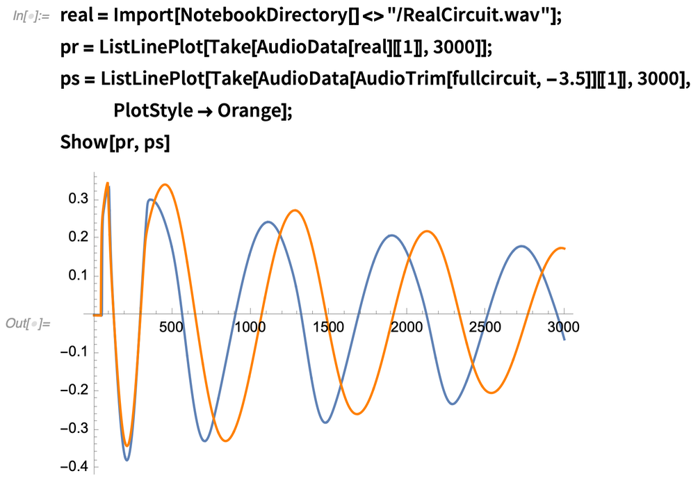
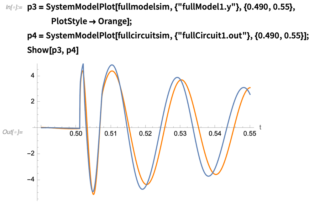
Great, lets talk fixed step solvers. How come you had to remove important transistor modelling from you 808 kick drum model? As shown in these diagram the shapes are different, as some transistor distortion of the filter is removed in both:
or
I’d love to be able to have a more detailed simulation, but it seems your methods are taking too much cpu to do this, so we can talk about it!
I suppose the better question is: why bother with Mathematica System Modeller in the first place if it’s hugely inefficient? Why not just use LTSpice or something like that? What does it actually do for you? I’ve found Mathematica solving pretty much pointless in my workflow, as the expressions it gives you are unwieldy and pretty much unusable for all but the smallest and simplest of matrices.
In the blog post I think I cover the reasons to remove/simplify the transistors: many of those are used as switches and can be replaced by simpler models: ideal switches or piecewise models. My opinion is that, if a semiconductor goes from zero to saturation (and vice-versa) in less than the time of one sample, then it does not worth having a detailed model.
In the blog post I also mention the problems with component variability when comparing simulation results against measurements. However I do not go into details on what can be considered an acceptable simulation. When creating an electrical model it is possible to perform a variability analysis, in this case, simulating the model changing the components within their tolerance margin. I used 1% resistors, and a mix of 1% and 5% capacitors. After performing a bunch of simulations with random values of each component (within their tolerance) it is possible to obtain a the acceptable limits. If the measurements fall inside those bands one can say that the model matches the real circuit according to the measurements. If you want to improve the confidence in your model, you will have to take (in this case) a bunch of 808 drum circuits, measure them all, and make sure that they fall in the bands.
It is not. I guess you are jumping to conclusions without having enough information or first-hand experience.
System Modeler is not only a circuit simulator. We can model multi-domain systems, like combinations of electrical, hydraulic, biological, chemical, mechanic, magnetic, etc. Trying to do that in LTSpice would be very difficult if not impossible.
If it does not adapt to your workflow it is fine. To mine it adapts very well. I use heavily the symbolic computations but I understand that some people prefer numeric computations. Mathematica requires some level of proficiency to do advanced stuff and some people is not willing to invest on learning it.
Well, now that you mention it, I prefer symbolic computations as well, that’s why I wrote an entire symbolic solver myself, since Mathematica was too slow to solve the complicated circuits I wanted to without compromising on detail. I did look into using it, but it ended up being quicker just to code my own in c++. Since I use Mathematica, and realise it does simplify small equations well, I did look into how it represents equations, and wrote my own n-ary tree symbolic expression solver and simplifier from scratch. I setup multiple systems of equations and solve them all symbolically, then run the solution through a simplification engine to pull out all common sub-expressions and other cpu saving pre-computations all automatically. Then either a c++ template / a python class / mathematica code / or julia code is generated directly from the spice like netlist. I view it as a very interesting optimisation problem to generate a symbolic solution with the fewest arithmetic operations possible.
I agree that it is an interesting approach. Specially if your problem is constrained, then it is possible to optimize it and make it fast.
Back in 2009 I wrote a SPICE-like simulator for a well known company. The reason why they needed one was because they require it to be fast, simpler and without any licensing. Since we had a constrained number of components and simplified transistor models that thing ran very fast. Customizing the tool to the problem results in very fast result.
In System Modeler we have our model compiler which is a custom symbolic manipulation engine that performs similar task to what you mention (that’s the team I work with). We take Modelica code and process it in order to get a DAE representation of the model. The resulting DAE is processed in order to find an efficient way of solving it and we generate C++ code to plug it with our solver. It can handle thousands of equations without breaking a sweat. The Modelica language is a complex beast so the compiler is a huge project.
That sounds more promising to me, thanks for going into some actually useful details! I’m a Mathematica customer, and I love the notebook approach, which is where the code and the diagrams and plots all live together in a live document that I can come back to later and pick up where I left off easy, since it is encourages self documentation, unlike c code or matlab etc.
I have a current Mathematic maintenance type license, I’ve downloaded a trial of System Modeler and the public ModelicaStandardLibrary_v4.0.0.zip.
I’ve grabbed your .zip download from the 808 page and can see at line 694 in DrumModeling.mo there is “model FullCircuit”. Just say I wanted to, without further manual optimisation, turn that into c++ code what are the basic steps to see a .h and .hpp or .cpp that solves that?
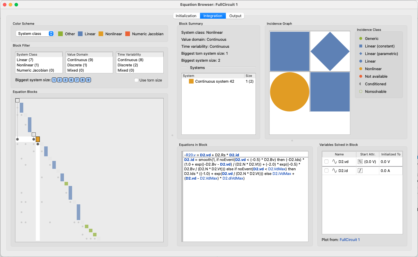
To see the generated code, once you simulate a model and you are in Simulation Center you can go to View->Generated Source Code. I have to warn you that it is not easy to take that code and plug it to other simulation backend. It is very customized and the equations are hard to extract without a lot of manual work. I recommend you to see the Equation Browser. You will find it in Tools->Equation Browser. There you can find an easier view of the equation blocks and the order in which they are solved.
This is an example of that view where I’m showing on of the blocks of non-linear equations that need to be solved for one of the semiconductors.
Other important thing is that the models in my blog post are made with the Modelica Standard Library 3.2.1 and they will not work out of the box in 4.0.0. We have a tool to migrate them but I don’t know if it’s released yet.
For reference my method involves defining the circuit as shown in the linked .cpp file, and then running my solver class to directly generate .h and .hpp template files, so the entire turnaround time between modifying the circuit and having it compiled as a module in VCV Rack is around 1-2 mins, and this goes up to around 5-20 mins if I enable more in-depth simplifications, or even longer if I want, but there isn’t much gain after around 10 mins.
I write each of the component models, which add entries into the sparse symbolic matrix, and then generate the required setup and non-linear evaluation code, and the solver computes the symbolic matrix solution, and then the optimiser makes it all run fast and spits out the final code.
In the CF100 I’m modelling the OTAs with a Boyle like input only differential npn transistor pair, then have diodes doing the clipping next to the filter capacitors to save on a few pnps, and the output BJT Darlington buffers do add a tiny bit of drive, but I’ve skipped this and just used perfect buffers with some dc offset since I couldn’t hear much difference because the internal of the OTAs did all the clipping / tone.
Ahh, I see, it looks like Modelica is built into the Wolfram System Modeler. @modlfo : So is the System Modeler a nice front end for Modelica? Basically it generates code that calls into Modelica to actually do the computation? I was hoping it would generate the code directly that did the simulation, not call a library to do the heavy lifting.
@brer_rabbit Probably this should be in its own thread to not distract from this great discussion with @andy-cytomic and @modlfo . This stuff is just stunning!! Do you plan to make it as a open source DIY project or a commercial one? Great stuff indeed @brer_rabbit !